Data platforms on Chameleon
You are an engineer at GourmetGram, a startup where users upload food photos, write captions, and interact through views, comments, and flags. GourmetGram is in a major growth phase, thanks in part to our previous infrastructure and MLOps work.
Now our manager wants to expand the platform with more ML features, and has suggested content moderation as a strong first use case for a new model. To make that possible, we need to build a data platform that supports both real-time decisions and reliable training data.
In this lab, we will build that platform progressively:
- First, we will use PostgreSQL to store core application state for users, images, comments, and flags.
- Then, we will expose API endpoints and run synthetic traffic generation so the system has realistic activity data.
- Next, we will add a real-time pipeline for streaming events and moderation triggers.
- After that, we will add a batch lakehouse layer with Iceberg tables for durable training data.
- Finally, we will train and deploy a moderation model and compare model-based decisions with heuristic decisions.
To run this lab, we should already have a Chameleon account, be part of a project, and have an SSH key uploaded to KVM@TACC.
Before we begin, open this experiment artifact on Trovi:
Then follow along with the published lab page:
Launch and set up a VM instance with python-chi
We will use the python-chi Python API to Chameleon to provision a VM instance.
We will execute the cells in this notebook inside the Chameleon Jupyter environment.
Run the following cell and make sure the correct project is selected.
# run in Chameleon Jupyter environment
from chi import server, context, lease, network
import chi, os, datetime

context.version = "1.0"
context.choose_project()
context.choose_site(default="KVM@TACC")
username = os.getenv("USER")  # all experiment resources will have this prefix
We will bring up an m1.xlarge flavor server with the CC-Ubuntu24.04 disk image.
Note: the following cell brings up a server only if we do not already have one with the same name, regardless of its error state. If we already have a server in ERROR state, delete it first in the Horizon GUI before running this cell.
First, we reserve the VM instance for 8 hours, starting now:
# run in Chameleon Jupyter environment
l = lease.Lease(f"lease-data-{username}", duration=datetime.timedelta(hours=8))
l.add_flavor_reservation(id=chi.server.get_flavor_id("m1.xlarge"), amount=1)
l.submit(idempotent=True)
# run in Chameleon Jupyter environment
l.show()
Now we can launch an instance using that lease:
# run in Chameleon Jupyter environment
s = server.Server(
    f"node-data-{username}",
    image_name="CC-Ubuntu24.04",
    flavor_name=l.get_reserved_flavors()[0].name,
)
s.submit(idempotent=True)
Then, we associate a floating IP with the instance:
# run in Chameleon Jupyter environment
s.associate_floating_ip()
In the output below, make a note of the floating IP assigned to the instance (in the “Addresses” row).
# run in Chameleon Jupyter environment
s.refresh()
s.show(type="widget")
By default, all connections to VM resources are blocked as a security measure. We need to attach one or more security groups to permit access over the Internet on specific ports.
The following security groups will be created (if they do not already exist in our project) and then added to our server. These include SSH, Jupyter, and the user-facing dashboards we will access throughout the lab:
# run in Chameleon Jupyter environment
security_groups = [
    {"name": "allow-ssh", "port": 22, "description": "Enable SSH traffic on TCP port 22"},
    {"name": "allow-8888", "port": 8888, "description": "Enable TCP port 8888 (Jupyter)"},
    {"name": "allow-8000", "port": 8000, "description": "Enable TCP port 8000 (FastAPI docs)"},
    {"name": "allow-8080", "port": 8080, "description": "Enable TCP port 8080 (Airflow UI)"},
    {"name": "allow-5050", "port": 5050, "description": "Enable TCP port 5050 (Adminer UI)"},
    {"name": "allow-8090", "port": 8090, "description": "Enable TCP port 8090 (Redpanda Console)"},
    {"name": "allow-8081", "port": 8081, "description": "Enable TCP port 8081 (Redis Insight)"},
    {"name": "allow-9001", "port": 9001, "description": "Enable TCP port 9001 (MinIO Console)"},
    {"name": "allow-3000", "port": 3000, "description": "Enable TCP port 3000 (Nimtable UI)"},
]
# run in Chameleon Jupyter environment
for sg in security_groups:
    secgroup = network.SecurityGroup(
        {
            "name": sg["name"],
            "description": sg["description"],
        }
    )
    secgroup.add_rule(direction="ingress", protocol="tcp", port=sg["port"])
    secgroup.submit(idempotent=True)
    s.add_security_group(sg["name"])

print(f"updated security groups: {[sg['name'] for sg in security_groups]}")
# run in Chameleon Jupyter environment
s.refresh()
s.check_connectivity()
Retrieve code and notebooks on the instance
Now, we can use python-chi to execute commands on the instance to set it up. We will start by retrieving the lab code and materials on the instance.
# run in Chameleon Jupyter environment
s.execute("git clone https://github.com/teaching-on-testbeds/data-platform-chi")
Set up Docker
Here, we install Docker on the instance.
# run in Chameleon Jupyter environment
s.execute("curl -sSL https://get.docker.com/ | sudo sh")
s.execute("sudo groupadd -f docker; sudo usermod -aG docker $USER")
Open an SSH session
Finally, open an SSH session on the server. From your local terminal, run:
ssh -i ~/.ssh/id_rsa_chameleon cc@A.B.C.D
where:
- in place of
~/.ssh/id_rsa_chameleon, substitute the path to your own key uploaded to KVM@TACC - in place of
A.B.C.D, use the floating IP address associated with your instance.
Initialize the application data layer
We will start with application data. In GourmetGram, this is the transactional data for users, images, comments, and flags, all of which supports the business logic and UI that real users interact with.
Our data repository will be PostgreSQL: it is great for application reads and writes, and for representing current state of the application
Here is a system view for the application phase (this notebook + the next notebook):
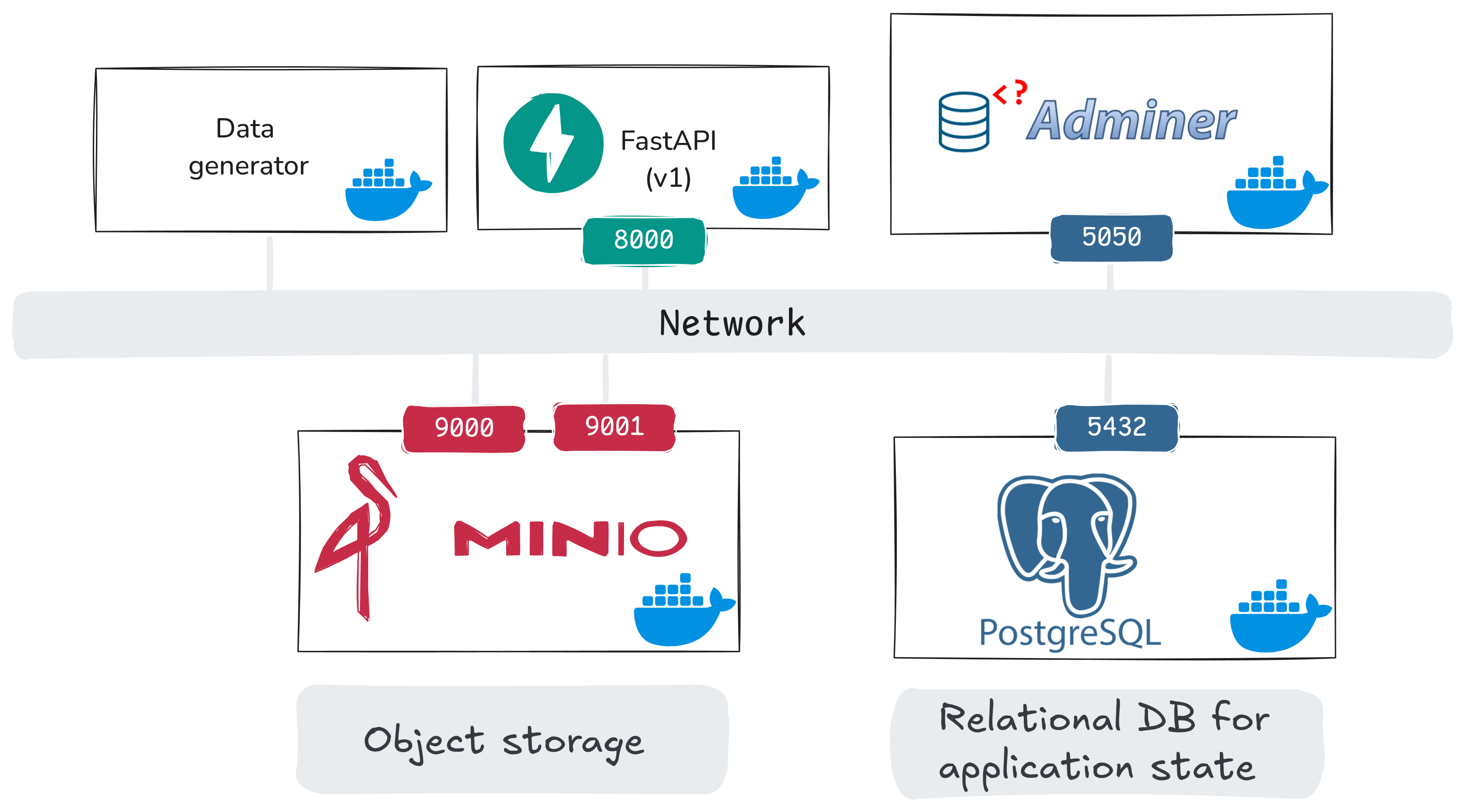
In this notebook, we bring up:
- PostgreSQL: relational database for application state
- Adminer: browser UI to inspect PostgreSQL tables
- MinIO + MinIO init: object storage for uploaded images, and an init job that sets up buckets
and prepare some database tables, but they will initially be empty. In the next notebook, we will add:
api_v1(FastAPI): application endpoints for users/uploads/comments/views/flagsdata_generator: synthetic client traffic into those endpoints- extract/transform helper services: one-time job, prepares the image samples that will be used for synthetic uploads
Before we start services, let’s inspect the PostgreSQL service definition in docker/docker-compose.yaml in more detail:
postgres:
  image: postgres:18
  container_name: postgres
  environment:
    POSTGRES_USER: user
    POSTGRES_PASSWORD: gourmetgram_postgres
    POSTGRES_DB: gourmetgram
  ports:
    - "5432:5432"
  volumes:
    - postgres_data:/var/lib/postgresql
    - ./init_sql:/docker-entrypoint-initdb.d
  healthcheck:
    test: [ "CMD-SHELL", "pg_isready -U user -d gourmetgram" ]
Here,
image: selects the Postgres version used in this lab.environment: sets database name and login credentials as environment variables. (We’ve hardcoded them for convenience, but in a real service you would not include these in the Compose file.)ports: maps container Postgres port to VM port5432. Other services will access it on that portvolumes: keeps database data persistent (postgres_data) across container restarts, and mounts initialization SQL files (./init_sql) which we will use to set up tables when Postgres comes up.healthcheck: lets dependent services wait until Postgres is ready.
Because ./init_sql is mounted into /docker-entrypoint-initdb.d, Postgres runs those SQL files on first initialization. For example, this images table definition comes from docker/init_sql/00_create_app_tables.sql:
CREATE TABLE IF NOT EXISTS images (
    id UUID PRIMARY KEY DEFAULT gen_random_uuid(),
    user_id UUID NOT NULL REFERENCES users(id),
    s3_url VARCHAR NOT NULL,
    source VARCHAR(32) NOT NULL DEFAULT 'user_upload',
    caption TEXT,
    category TEXT,
    created_at TIMESTAMPTZ DEFAULT NOW(),
    deleted_at TIMESTAMPTZ,
    views INTEGER DEFAULT 0,
    CHECK (source IN ('user_upload', 'synthetic', 'import'))
);
This schema gives each image a durable identifier, links it to a user (user_id), stores object location (s3_url), tracks app state for the image (views), and includes governance-oriented fields (source, deleted_at).
From your SSH session on the Chameleon VM, start only the database and the Adminer UI:
# run on node-data
docker compose -f /home/cc/data-platform-chi/docker/docker-compose.yaml up -d postgres adminer
Check that both services are running:
# run on node-data
docker ps
You should see postgres and adminer in running (or healthy) state.
Browse PostgreSQL in the UI
Adminer is a browser-based UI for Postgres. Open it in your browser:
http://A.B.C.D:5050
where A.B.C.D is the floating IP address associated with your instance.
Use the following login values:
- System: PostgreSQL (use the drop-down to change it!)
- Server:
postgres - Username:
user - Password:
gourmetgram_postgres - Database:
gourmetgram
Then click Login.
After login, inspect the core application tables:
- Click one table name (for example
users). - Click “Show structure” to see the schema, and “Select data” to browse the data. Currently, these tables will all be empty.
- Repeat for
images,comments,flags, andmoderation.
Eventually, our application state will leave in these tables as follows:
users: account-level application state. This includes ToS fields for governance checks,country_of_residencefor regional policy slices, andis_test_accountto filter synthetic/internal accounts used for testing from analysis.images: image records plus metadata. Thesourcefield helps us separate user content from synthetic content, anddeleted_atallows for soft deletion.comments: user-generated text attached to images.moderator_hiddenandmoderator_action_idlet us track when content is hidden and which moderation action caused it.flags: user reports of problematic content.review_status,resolved_at, andmoderation_action_idare populated during the review workflow.moderation: moderation outcomes for images/comments/accounts.risk_scoreis a risk value attached to the item by a model or a heuristic,model_versionidentifies which model produced it, andinference_request_idlinks related records from one inference request, so that we can audit ML-assisted moderation outcomes.
Prepare object storage for uploads
Let’s also set up MinIO and create the required buckets. MinIO will store images that are uploaded to GourmetGram - we saw in the PostgreSQL images table that there is a field where we will put the image’s location in the object store.
Here’s the relevant compose section:
minio:
  image: minio/minio:RELEASE.2025-09-07T16-13-09Z
  container_name: minio
  command: server /data --console-address ":9001"
  environment:
    MINIO_ROOT_USER: admin
    MINIO_ROOT_PASSWORD: gourmetgram_minio
  ports:
    - "9000:9000"
    - "9001:9001"

minio-init:
  image: minio/mc:RELEASE.2025-08-13T08-35-41Z-cpuv1
  container_name: minio-init
  depends_on:
    minio:
      condition: service_healthy
  command: |
    mc alias set myminio http://minio:9000 admin gourmetgram_minio
    mc mb --ignore-existing myminio/gourmetgram-datalake
    mc mb --ignore-existing myminio/gourmetgram-images
Note that there is a minio-init job that creates two buckets, one for images and one that is used later in the lab.
Run:
# run on node-data
docker compose -f /home/cc/data-platform-chi/docker/docker-compose.yaml up -d minio minio-init
Open the MinIO console at http://A.B.C.D:9001 (use your floating IP in place of A.B.C.D). Log in with the credentials:
- Username:
admin - Password:
gourmetgram_minio
After login:
- Click Object Browser in the left menu.
- Confirm that the bucket
gourmetgram-imagesexists. (It was created by the minio-init job.) - Click the bucket name and verify it is currently empty.
It does not yet have any images - but it will soon. In the next part, we will turn on API endpoints and synthetic traffic so that PostgreSQL tables and MinIO objects are populated with realistic application activity.
Bring up dummy endpoints and synthetic traffic
Next, we will stand up a simple application layer for GourmetGram: “dummy” API endpoints for users, uploads, comments, views, and flags, that will persist data to our PostgreSQL database (and, images to the object storage service). Then we will run a synthetic traffic generator against those endpoints.
This gives us realistic application activity in PostgreSQL before we add more advanced platform pieces.
The data flow we are setting up in this phase is illustrated in the following diagram:
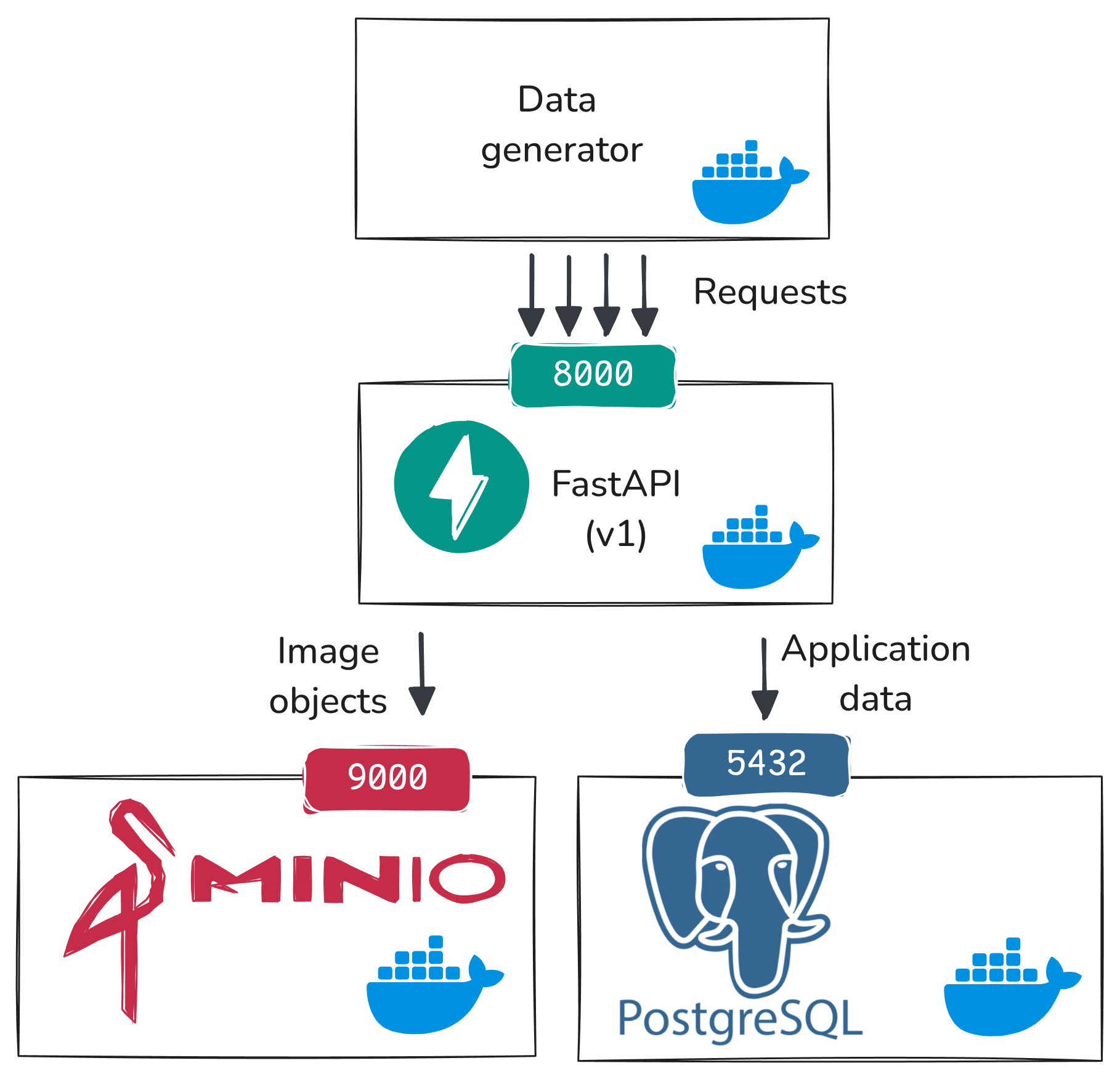
At this stage:
data_generatorsends HTTP requests toapi_v1endpointsapi_v1writes application state to PostgreSQL (users,images,comments,flags)api_v1writes uploaded image objects to MinIO
This is the baseline flow we will build on in the rest of the experiment.
Step 1: Prepare image data artifacts
At this point, PostgreSQL/Adminer and MinIO/buckets are already running from the previous notebook.
Now, prepare image data (the Food-11 dataset). The synthetic data generator will randomly select existing food images from this data to send to our endpoint.
The extract-data and transform-data steps download and organize the Food-11 dataset used by the generator.
# run on node-data
docker compose -f /home/cc/data-platform-chi/docker/docker-compose.yaml up -d \
  extract-data transform-data
Step 2: Start dummy API endpoints
Now bring up the API service:
# run on node-data
docker compose -f /home/cc/data-platform-chi/docker/docker-compose.yaml up -d api_v1
and use
# run on node-data
docker ps
to confirm it is running.
To see how these endpoints work and what type of input they accept, open the docs in your browser (substituting your floating IP in place of A.B.C.D):
http://A.B.C.D:8000/docs
In the docs page:
- Click one endpoint row (for example
POST /upload/). - Click Try it out.
- Review the example request fields.
- Click Cancel (or do not execute) and repeat for other endpoints.
Take screenshots for later reference.
These endpoints are “dummy” in the sense that we haven’t built any application logic on top of them, but they model the core application workflow we need for the rest of the lab.
Step 3: Start synthetic traffic generation
Now, start the synthetic data generator:
# run on node-data
docker compose -f /home/cc/data-platform-chi/docker/docker-compose.yaml up -d data_generator
and once it is up, watch its logs:
# run on node-data
docker logs -f generator
You should see activity like user creation, image uploads, comments, views, and flags.
Go back to Adminer (http://A.B.C.D:5050) and log in with:
- System:
PostgreSQL(use drop-down to change it) - Server:
postgres - Username:
user - Password:
gourmetgram_postgres - Database:
gourmetgram
Then, confirm that records are accumulating in the comments, flags, images, and users tables, and that in the images table, some images are accumulating views. (Click on a table, then “Select data” to see the data in the table.)
Take screenshots of Adminer table views for comments, flags, images, and users as well as example rows from each table.
In MinIO (http://A.B.C.D:9001):
- Click Object Browser.
- Click
gourmetgram-images. - Confirm uploaded files are appearing. You can click on file and then choose the “Preview” option in the sidebar to see the image.
Adding a real-time pipeline
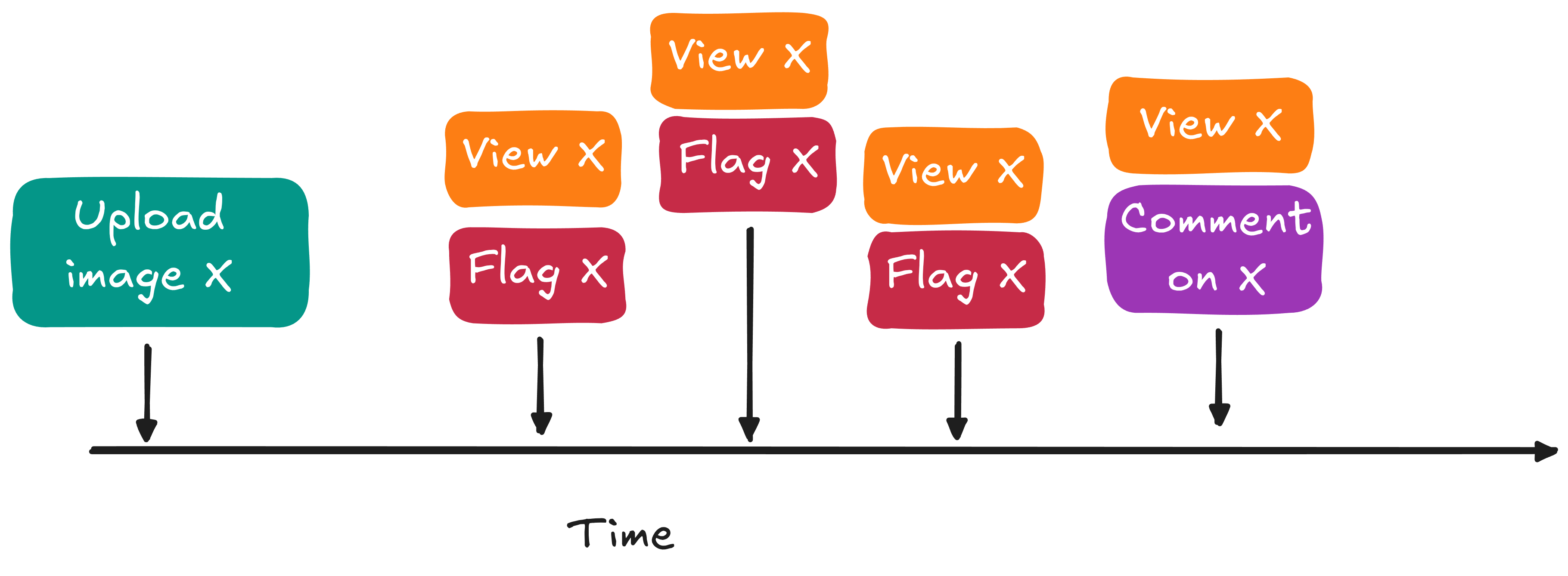
Our goal is to introduce ML into content moderation. We want to train a model that will assign risk scores to content, so that human moderators will know which content is likely to be harmful and should be reviewed quickly. (For example: a user-uploaded image that contains violence and disturbing content, instead of delicious food items.)
We will score each image immediately when it is uploaded. However, since more information becomes available as time goes on (e.g. flags, comments, etc.) we will also want to re-score each image at additional anchor times, using signals like:
- how many views arrived recently
- how many comments arrived recently
- how many flags arrived recently
Those time-anchored signals will be needed in two places:
- inference: decide now whether content is safe, or whether it needs urgent review
- training: help our model understand how to do better, given both the information known at inference time and the eventual moderation decision
Our current data repository, PostgreSQL is the transactional system of record for current application state, but querying it directly is not appropriate for inference or for training. First of all, using the serving database to compute features for real-time inference and for training will add extra load and potentially degrade the actual GourmetGram service. Second, the database tells us application state e.g. total views at the current time, but it doesn’t give us the time-anchored views that we will need for training (what was the recent view count at upload time? at 5 minutes after upload time? at 30 minutes after upload time?)
So we keep PostgreSQL for durable application state, and add additional data systems to support real-time inference and training. In this section, we will focus on the real-time data flow for inference.
Here is our system view for the real-time phase:
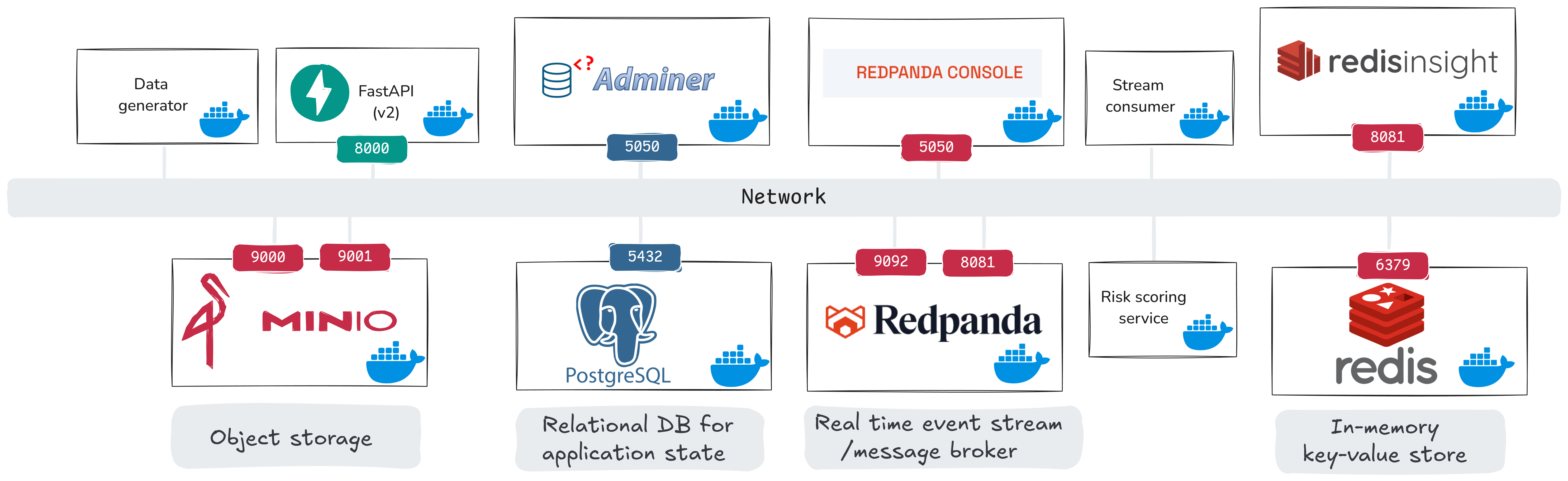
From the previous phase, we already have data_generator, api_v1, PostgreSQL, and MinIO. The newly introduced components are:
api_v2: streaming-enabled API version (also publishes events to Redpanda), replacesapi_v1- Redpanda + Redpanda Console: event stream broker and UI
- Redis + Redis Insight: in-memory feature store and UI
stream_consumer: a custom service that computes rolling windows and emits moderation requestsrisk_scoring_service: a custom service that consumes moderation requests and writes moderation scores
The key Compose blocks for Redpanda and Redis are:
redpanda:
  image: docker.redpanda.com/redpandadata/redpanda:v25.3.7
  container_name: redpanda
  command:
    - redpanda
    - start
    - --kafka-addr internal://0.0.0.0:9092,external://0.0.0.0:19092
    - --advertise-kafka-addr internal://redpanda:9092,external://localhost:19092
    - --pandaproxy-addr internal://0.0.0.0:8082,external://0.0.0.0:18082
    - --advertise-pandaproxy-addr internal://redpanda:8082,external://localhost:18082
    - --schema-registry-addr internal://0.0.0.0:8081,external://0.0.0.0:18081
    - --rpc-addr redpanda:33145
    - --advertise-rpc-addr redpanda:33145
    - --smp 1
    - --memory 1G
    - --mode dev-container
    - --set redpanda.log_retention_ms=2592000000
    - --set redpanda.log_segment_ms=3600000
  ports:
    - "18081:18081"
    - "18082:18082"
    - "19092:19092"
    - "19644:9644"
  healthcheck:
    test: [ "CMD-SHELL", "rpk cluster health | grep -E 'Healthy:.+true' || exit 1" ]
    interval: 15s
    timeout: 3s
    retries: 5

redis:
  image: redis:7-alpine
  container_name: redis
  ports:
    - "6379:6379"
  volumes:
    - redis_data:/data
  healthcheck:
    test: [ "CMD", "redis-cli", "ping" ]
    interval: 5s
    timeout: 3s
    retries: 5
  command: redis-server --appendonly yes
The stream consumer Kafka wiring comes from this Compose block:
stream_consumer:
  environment:
    - KAFKA_BOOTSTRAP_SERVERS=redpanda:9092
    - KAFKA_CONSUMER_GROUP=gourmetgram-stream-consumer
    - KAFKA_TOPICS=gourmetgram.views,gourmetgram.comments,gourmetgram.uploads,gourmetgram.flags
    - MODERATION_TOPIC=gourmetgram.moderation_requests
And in code, the consumer is initialized with those settings and subscribes to all source topics:
self.consumer = KafkaConsumer(
    *config.kafka_topics,
    bootstrap_servers=config.kafka_bootstrap_servers,
    group_id=config.kafka_consumer_group,
    auto_offset_reset='earliest',
    enable_auto_commit=config.consumer_auto_commit,
    max_poll_records=config.consumer_max_poll_records,
    value_deserializer=lambda m: json.loads(m.decode('utf-8')),
)
The stream consumer is where API events are transformed into rolling features and moderation requests. In simplified form:
for event in kafka_consumer.poll():
    if event["event_type"] == "view":
        process_view_event(event)
    elif event["event_type"] == "comment":
        process_comment_event(event)
    elif event["event_type"] == "flag":
        process_flag_event(event)
and
redis.zadd("image:<id>:views:5min", score=timestamp, member=member)
views_5min = zcount("image:<id>:views:5min")
if views_5min >= VIRAL_THRESHOLD:
    publish("gourmetgram.moderation_requests", {"image_id": image_id, "trigger": "viral"})
The risk scoring service (heuristic mode in this stage) reads each moderation request, builds features, and computes a risk score from simple rules:
if total_flags > 0:
    score += 0.4
if comments_5min > 10:
    score += 0.3
if views_5min > 100:
    score += 0.2
score = min(score, 1.0)
Then it persists that score:
INSERT INTO moderation (target_type, target_id, inference_mode, model_version, risk_score, trigger_type)
VALUES ('image', :image_id, 'heuristic', NULL, :risk_score, :trigger);
Here is the updated data flow including the real-time pipeline:
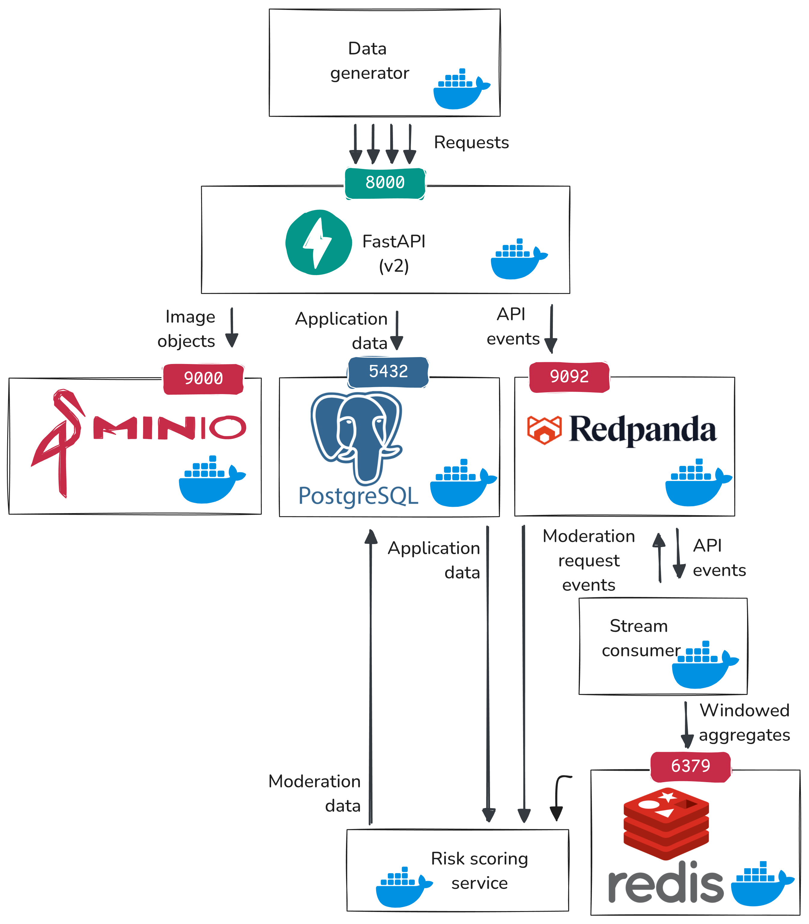
- The data generator sends synthetic user activity to our API endpoints (uploads, views, comments, flags).
api_v2handles each request and does two writes:- write current application state to PostgreSQL (for example, increment
images.views) - emit an event record to Redpanda
- write current application state to PostgreSQL (for example, increment
- Redpanda is the message broker. It stores those event records in ordered topics, so downstream services can read a time-ordered stream of what happened.
- A stream consumer reads those topics, keeps rolling counts (for example, recent views/comments/flags), and decides if an inference request should be triggered based on some heuristic rules.
- The stream consumer writes the rolling features to Redis (fast in-memory lookup store) and/or publishes a moderation inference request event to Redpanda.
- The risk scoring service reads the moderation inference request from Redpanda, fetches the latest rolling features from Redis and other features from PostgreSQL, and computes a risk score.
- The risk scoring service writes its output to PostgreSQL (
moderationtable), so that it can be used by application logic.
So PostgreSQL keeps durable application and moderation records, Redpanda carries ordered event history, Redis holds the latest fast-changing features, and inference consumes those features to make decisions.
Before we run the real-time services, we should define the inference inputs exactly.
For each moderation request, the risk scoring service builds a 29-dimensional feature vector:
- Temporal (4):
time_since_upload_seconds,hour_of_day,day_of_week,is_weekend - Window aggregates (6):
views_5min,views_1hr,comments_5min,comments_1hr,flags_5min,flags_1hr - Flag count (1):
total_flags - Derived engagement (3):
view_velocity_per_min,comment_to_view_ratio,recent_engagement_score - Content features (2):
caption_length,has_caption - User features (2):
user_image_count,user_age_days - Category one-hot (11):
category_Bread,category_Dairy,category_Dessert,category_Egg,category_Fried,category_Meat,category_Noodles,category_Rice,category_Seafood,category_Soup,category_Veggie
where:
- Redis provides rolling window counts, which are also used for the derived engagement metrics.
- PostgreSQL provides image/user metadata needed to construct temporal, content, and user features.
In the future, we might add fused image embeddings to this input. For now, inference uses only the tabular behavioral and metadata features listed above.
Step 1: Start the real-time services
Stop api_v1 and the synthetic generator so we can switch into the real-time stage:
# run on node-data
docker compose -f /home/cc/data-platform-chi/docker/docker-compose.yaml stop data_generator
docker compose -f /home/cc/data-platform-chi/docker/docker-compose.yaml stop api_v1
Now start api_v2, the message broker, stream processing, and the risk scoring service:
# run on node-data
docker compose -f /home/cc/data-platform-chi/docker/docker-compose.yaml up -d \
  api_v2 redpanda redpanda-console redis redisinsight stream_consumer risk_scoring_service
and check that services are running with
# run on node-data
docker ps
Quick check that the running API is the streaming-enabled version:
# run on node-data
curl -s http://127.0.0.1:8000/docs
Open http://A.B.C.D:8000/docs, then:
- Click
GET /health. - Click Try it out.
- Click Execute.
- In the JSON response body, confirm
kafka_enabledis present.
Then, bring up the data generator:
# run on node-data
docker compose -f /home/cc/data-platform-chi/docker/docker-compose.yaml up -d data_generator
Now that services are up, we will trace one “suspicious” image through this path: API event -> Redpanda topics -> stream consumer windowing in Redis -> moderation request -> risk scoring -> moderation row in PostgreSQL.
Step 2: Inspect the real-time data flow
Open these UIs (with your own floating IP):
- Redpanda Console:
http://A.B.C.D:8090 - Redis Insight:
http://A.B.C.D:8081
(Neither Redpanda Console nor Redis Insight requires a username/password in our configuration.)
Our updated API service persists application state to PostgreSQL, but also sends events to Redpanda, which keeps our event stream.
In Redpanda Console:
- Click Topics in the left menu.
- Click
gourmetgram.viewsand confirm that messages appear in the messages panel. - Repeat for
gourmetgram.comments,gourmetgram.flags, andgourmetgram.uploads.
You should see events arriving in:
gourmetgram.viewsgourmetgram.commentsgourmetgram.flagsgourmetgram.uploads
Note that “views” in particular are not saved individually in PostgreSQL - only a cumulative count - because they were not needed for application state. But now, downstream services that require individual view counts or aggregated view counts over time windows can get them from the event stream.
Watch the service logs of the stream consumer:
# run on node-data
docker logs -f stream-consumer
and in another terminal:
# run on node-data
docker logs -f risk-scoring-service
Step 3: Force one concrete inference example
In a production system, we would usually emit a moderation request for every new upload, so the risk scoring service can score content immediately from metadata features (for example caption/content metadata and uploader context), then re-score later as engagement signals arrive.
In this lab, to keep the flow simple and easy to trace, we only emit gourmetgram.moderation_requests when a heuristic real-time trigger fires: bursts in views/comments/flags.
Trigger a synthetic viral burst so that one moderation request is guaranteed to fire:
# run on node-data
docker compose -f /home/cc/data-platform-chi/docker/docker-compose.yaml run --rm --no-deps \
  -e GENERATOR_MODE=simulate_viral \
  -e GENERATOR_BURST_VIEWS=110 \
  -e GENERATOR_BURST_COMMENTS=8 \
  -e GENERATOR_BURST_FLAGS=2 \
  data_generator
This publishes a burst of view events for one real image. Within a few seconds, the stream consumer should publish a moderation request, and the risk scoring service should produce a decision.
The simulation should print something like:
Simulating viral burst for image: 123e4567-e89b-12d3-a456-426614174000
with an image ID. Copy the image ID printed by the script. We will call this value IMAGE_ID.
Step 4: Trace one viral item through the real-time flow
Now, you will trace this item through the real-time data flow, and you will take screenshots at each stage.
In the Redpanda Console, which is open at http://A.B.C.D:8090, let’s follow the same IMAGE_ID across services:
First, in Redpanda Console, click Topics -> gourmetgram.views, then use the message filter/search box to search for IMAGE_ID and confirm burst view events arrived.
The stream consumer will have written aggregates to Redis. Open Redis Insight (http://A.B.C.D:8081), then in the Filter by Key Name or Pattern box type: image:IMAGE_ID* (include the trailing *). Do this quickly after running the viral burst, because rolling-window keys are time-based and old entries are cleaned up.
In Redis Insight, expand the tree image -> IMAGE_ID -> (views, comments, flags). You will see window keys such as 1hr and sometimes 5min.
To interpret what you see in Redis Insight for a sorted-set key (for example image:IMAGE_ID:flags:1hr):
- Member is the stored event token. In this lab, it is a string like
flag:<event_timestamp>:<random_suffix>. Each member corresponds to one event that happened for this image. - Score is the event timestamp (Unix time, seconds). Redis uses this numeric score to keep members ordered by time and to support window queries.
- The sorted set itself is the “value” for that key. So for sorted sets, the value is not one scalar number; it is the collection of
(member, score)pairs. - The Length shown near the top of the key details panel is the current number of members in that set (that is, event count currently in the window).
- TTL is how long until Redis expires the key. Because these are rolling windows, keys naturally age out.
For keys like total_flags, total_comments, and total_views, the key type is STRING; in that case the value is a scalar counter.
This image will have triggered the stream consumer to write an event to moderation_requests. In Redpanda Console, click gourmetgram.moderation_requests and verify at least one message includes the same IMAGE_ID.
The risk scoring service will have read the request from Redpanda, applied a heuristic to compute a risk score, and produced an output. In risk scoring logs (docker logs -f risk-scoring-service), confirm the scoring request and stored moderation output for the same IMAGE_ID.
In Adminer (http://A.B.C.D:5050), log in with PostgreSQL / postgres / user / gourmetgram_postgres / gourmetgram, then confirm the same IMAGE_ID appears in target_id for a row in the moderation table.
Persist aggregated history to Iceberg
In the real-time stage, we built low-latency features from streaming events. That is good for online risk scoring, but training needs durable history that we can recompute consistently.
In this lab design, reconstructing view-related history from PostgreSQL is effectively impossible, because we do not store every raw view event there. PostgreSQL keeps current application state (for example total view counters), not complete per-view event history.
For comments and flags, retrospective counting from PostgreSQL is possible in principle. But we still prefer not to depend on that for training, because repeated time-window queries over large tables are expensive and can drift from the online feature logic.
This creates a model-training problem: we want feature values at arbitrary anchor times after upload (for example at upload time, +5 minutes, +30 minutes), but current-state tables alone do not reliably provide that.
So in this stage, we persist aggregated event history to Iceberg tables. We will materialize window aggregates at 5-minute intervals and use those durable aggregates as a stable source for training features.
Step 1: Start batch workflow services (Airflow)
We will use Airflow to orchestrate batch jobs that write to Iceberg. Bring up Airflow, along with Nimtable for viewing Iceberg tables:
# run on node-data
docker compose -f /home/cc/data-platform-chi/docker/docker-compose.yaml up -d \
  airflow-init airflow-webserver airflow-scheduler nimtable nimtable-web
The first startup can take a while. We use Airflow to orchestrate data workflows, and the Airflow image must include libraries for Iceberg and storage/database access (for example PyIceberg, Arrow, and related clients). That setup happens during the container image build, so initial bring-up is slower than the earlier services.
Open Airflow:
http://A.B.C.D:8080- username:
admin - password:
gourmetgram_airflow
After login:
- Click DAGs in the top navigation if you are not already on the DAG list page.
- Confirm you can see both pipeline DAGs:
redpanda_event_aggregationmoderation_training
At this point they may appear paused (toggle off). That is expected before we trigger runs in the next steps.
Step 2: Run event aggregation DAG first
The redpanda_event_aggregation DAG reads views, comments, and flags events from Redpanda, groups them into 5-minute windows, and writes those window counts to Iceberg tables in event_aggregations.
By default, this DAG is scheduled hourly (every hour on the hour). In production we would normally let the scheduler run it at those boundaries, but in this lab we trigger it early so we can see the full flow immediately.
This DAG also keeps a watermark in an Airflow Variable (redpanda_event_aggregation_checkpoint) using Kafka offsets per topic partition. On the first run, if that Variable does not exist yet, the DAG performs a historical backfill from earliest available offsets. After a successful run, it saves the next offsets as the new watermark so later runs continue incrementally.
In Airflow UI:
- Open DAG
redpanda_event_aggregation - Trigger a run by clicking the ▶
- Open the DAG run (for example from Recent Tasks/Graph) and wait until tasks are green (success).
If this is your first time running a DAG in Airflow, inspect it step by step:
- Open the DAG, then click Graph to see task order and dependencies.
- Click one task box (for example
consume_and_aggregate_events). - In the task popup, click Logs to open that task’s execution log.
- Repeat for each task (
write_view_windows,write_comment_windows,write_flag_windows,commit_checkpoint) so you can see what each step read/wrote. - Use Grid view to quickly check retries, durations, and final status across all tasks in the run.
This DAG is structured as:
dag = DAG(
    'redpanda_event_aggregation',
    schedule_interval=timedelta(hours=1),
    catchup=False,
)

t1_consume >> t2_write_views >> t3_write_comments >> t4_write_flags >> t5_commit_checkpoint
Watermark/backfill logic in this DAG is:
CHECKPOINT_VAR = "redpanda_event_aggregation_checkpoint"

checkpoint = Variable.get(CHECKPOINT_VAR, default_var=None, deserialize_json=True)
if checkpoint is None:
    # First run: historical backfill
    start_offsets = consumer.beginning_offsets(partitions)
else:
    # Incremental runs: resume from saved watermark
    start_offsets = checkpoint["offsets"]

# Freeze a run boundary so this run is deterministic
end_offsets = consumer.end_offsets(partitions)

# Consume [start_offset, end_offset) for each topic partition
# ...aggregate into 5-minute windows...

# Only after all Iceberg writes succeed:
Variable.set(CHECKPOINT_VAR, {"offsets": next_offsets}, serialize_json=True)
Here:
t1_consume: readsviews/comments/flagsevents from the current watermark up to this run boundary and bins them into 5-minute windows.t2_write_views,t3_write_comments,t4_write_flags: write those windowed aggregates to Iceberg tables.t5_commit_checkpoint: saves the next Kafka offsets to the Airflow Variable watermark after all writes succeed.
This DAG reads streaming events and writes 5-minute aggregate windows to Iceberg tables.
After this DAG succeeds, we should be able to confirm new Iceberg window tables:
event_aggregations.view_windows_5minevent_aggregations.comment_windows_5minevent_aggregations.flag_windows_5min
Check these in Nimtable: Open http://A.B.C.D:3000 and log in (admin / gourmetgram_nimtable).
In Nimtable, connect the Iceberg catalog, which is hosted in PostgreSQL:
- From the left sidebar, click Catalogs.
- Click Add Catalog -> Connect Catalog.
- Fill in:
- Connection Method:
JDBC + S3 - Catalog Name:
gourmetgram - Catalog Endpoint:
jdbc:postgresql://postgres:5432/iceberg_catalog - Warehouse:
s3://gourmetgram-datalake/warehouse - S3 Endpoint:
http://minio:9000 - Access Key:
admin - Secret Key:
gourmetgram_minio
- Connection Method:
- Open Advanced Options and add:
jdbc.user=userjdbc.password=gourmetgram_postgres
- Click Connect Catalog.
Then,
- Open Catalogs ->
gourmetgram. - Open namespace
event_aggregations. - Confirm the three
*_windows_5mintables are visible.
Take screenshots for later reference.
We are just browsing a catalog of data that is in the lakehouse, but the underlying storage is in MinIO. To see the underlying storage right after this Redpanda aggregation run:
- Open MinIO Console at
http://A.B.C.D:9001and log in (admin/gourmetgram_minio). - Click Object Browser, then open bucket
gourmetgram-datalake. - Open folder
warehouse/event_aggregations/and then one table folder such asview_windows_5min/. - Open
data/to see Parquet files that store the data. - Open
metadata/to see Iceberg metadata files (schemas, snapshots, file manifests).
Take screenshots for later reference.
Also inspect the watermark Variable in PostgreSQL via Adminer:
- Open Adminer at
http://A.B.C.D:5050. - Login with:
- System:
PostgreSQL - Server:
postgres - Username:
user - Password:
gourmetgram_postgres - Database:
airflow
- System:
- Open table
variable. - Click Select data.
- Add filter
key = redpanda_event_aggregation_checkpoint. - Click Select.
How to interpret the row:
id: internal primary key for this Airflow Variable row.key: Variable name (redpanda_event_aggregation_checkpoint).val: stored Variable value.description: optional note (oftenNULL).is_encrypted: whether Airflow encryptedvalwith its Fernet key.
Assuming is_encrypted is 1, so val appears as encrypted text in Adminer. To view the decoded JSON watermark payload (per-topic-partition offsets), query through Airflow itself:
# run on node-data
docker exec airflow-webserver airflow variables get redpanda_event_aggregation_checkpoint
Step 3: Run main training-data DAG
The moderation_training DAG builds the model-training dataset. It reads application data from PostgreSQL, joins in the 5-minute Iceberg aggregates we just produced, computes training features at multiple decision points, and writes the final dataset to Iceberg (moderation.training_data).
This DAG is scheduled daily. In normal operation we would let the daily schedule handle it, but in this lab we trigger it now so we can validate the full batch path end to end.
Its task flow is:
t1_extract_data >> t2_transform_features >> t3_load_iceberg
Here:
t1_extract_data: snapshotsusers,images,comments, andflagsfrom PostgreSQL into MinIO raw parquet paths.t2_transform_features: applies governance filters, combines application snapshots with Iceberg window tables (event_aggregations.*_windows_5min), and computes training features and labels.t3_load_iceberg: writes the resulting training dataset to Iceberg tablemoderation.training_data.
In t2_transform_features, we also enforce training data policy by only selecting eligible candidates for training. For example:
# examples from the DAG logic
# exclude test accounts
uploader_is_test = images['is_test_account'].fillna(False)
# exclude content from minors
uploader_is_child = images['year_of_birth'].notna() & (
    (images['created_at'].dt.year - images['year_of_birth']) < 18
)
# exclude deleted content
image_is_deleted = images['deleted_at'].notna()

eligible_images = images[(~uploader_is_test) & (~uploader_is_child) & (~image_is_deleted)]
We apply similar policy filters for comment/flag data, then create labels and features from the filtered data.
Although it is not implemented in this lab, we should think about what would happen if content is deleted after it already entered
moderation.training_data. We do not need a full table rebuild: Iceberg supports row-level correction workflows through snapshot updates: the pipeline can maintain exclusion keys (for example deletedimage_idvalues), then execute an IcebergDELETEor equivalent rewrite that removes matching rows in a new snapshot. Training readers use the latest snapshot, so excluded rows are no longer visible in current scans while table history is still preserved.
In Airflow UI:
- Open DAG
moderation_training - Trigger a run
- Open the run and wait until tasks are green (success).
This builds the training dataset by combining application data and windowed aggregates, then writes output to Iceberg.
After this DAG succeeds, verify the training table in Nimtable and MinIO.
In Nimtable:
- Open
http://A.B.C.D:3000and log in (admin/gourmetgram_nimtable). - Open Catalogs ->
gourmetgram. - Open namespace
moderation. - Open table
training_data. - Confirm schema and preview rows are visible.
In MinIO:
- Open
http://A.B.C.D:9001and log in (admin/gourmetgram_minio). - Open bucket
gourmetgram-datalake->warehouse/moderation/training_data/. - Confirm both
data/andmetadata/folders contain files. - Optionally compare timestamps to confirm new files were written by this run.
Train a moderation model from Iceberg
In the previous stage, we created moderation.training_data as an Iceberg table. Now can we use that table to train a model. An inference service with this model could potentially replace the heuristic “risk scoring service” that we introduced in the real time data pipeline.
We are going to train a classifier in Python with scikit-learn: we will read Iceberg tables through PyIceberg, then trains a logistic regression incrementally using an SGDClassifier.
Run this on node-data:
# run on node-data
docker compose -f /home/cc/data-platform-chi/docker/docker-compose.yaml up -d --build jupyter
The jupyter service in compose is:
jupyter:
  build:
    context: ../model_training
    dockerfile: Dockerfile
  container_name: jupyter
  ports:
    - "8888:8888"
  environment:
    - PYICEBERG_CATALOG__GOURMETGRAM__TYPE=sql
    - PYICEBERG_CATALOG__GOURMETGRAM__URI=postgresql+psycopg2://user:gourmetgram_postgres@postgres:5432/iceberg_catalog
    - PYICEBERG_CATALOG__GOURMETGRAM__S3__ENDPOINT=http://minio:9000
    - PYICEBERG_CATALOG__GOURMETGRAM__S3__ACCESS_KEY_ID=admin
    - PYICEBERG_CATALOG__GOURMETGRAM__S3__SECRET_ACCESS_KEY=gourmetgram_minio
    - PYICEBERG_CATALOG__GOURMETGRAM__WAREHOUSE=s3://gourmetgram-datalake/warehouse
  volumes:
    - ../model_training/workspace:/home/jovyan/work
Here,
builduses the Jupyter image frommodel_training/Dockerfile.portsexposes notebook UI on8888.PYICEBERG_CATALOG__...points PyIceberg at the SQL catalog in PostgreSQL and warehouse files in MinIO.volumesmountsmodel_training/workspaceinto/home/jovyan/work, so notebooks and saved artifacts persist in the lab directory.
After the service is up, get the Jupyter token:
# run on node-data
docker exec jupyter jupyter server list
Open the URL in your local browser, replacing localhost with your floating IP:
http://A.B.C.D:8888/tree?token=...
Then, in Jupyter:
- Open
training.ipynb. - Run cells top to bottom.
- Confirm training completes successfully.
The notebook uses PyIceberg to load data from the lakehouse, e.g.:
from pyiceberg.catalog import load_catalog

catalog = load_catalog("gourmetgram")
table = catalog.load_table("moderation.training_data")
Note that it does not have to specify the exact location in S3 where the data is saved - it finds out from the catalog.
We don’t have a lot of data, because we haven’t been running our “service” very long! But we consider that in the future, we will have a large training data set that does not fit in memory. So, we stream Arrow batches and train incrementally:
scanner = table.scan()
batches = scanner.to_arrow_batch_reader()

for batch in batches:
    df_batch = batch.to_pandas()
    model.partial_fit(X_batch, y_batch, classes=[0, 1])
Note thatIceberg also gives us dataset versioning for training reproducibility. Every table write creates a new snapshot. Before training, we can record the snapshot id for moderation.training_data and save it with model artifacts. Later, we can point to the exact snapshot used for that model version.
catalog = load_catalog("gourmetgram")
table = catalog.load_table("moderation.training_data")

snapshot_id = table.metadata.current_snapshot_id
print(f"Training from Iceberg snapshot: {snapshot_id}")
That means model version N can be traced back to a specific Iceberg snapshot, not just a vague time window.
At the end of the notebook, we save artifacts locally in the mounted workspace. Look in the models directory and confirm these files exist:
model.joblibscaler.joblibencoder.joblibmetadata.json
Open metadata.json and note snapshot_id: this is the exact Iceberg snapshot used for the training run.
Save metadata.json for later reference.
Delete and release resources
At the end of the lab, we delete the Chameleon server and lease so we do not leave compute reserved.
We will execute the next cells in the Chameleon Jupyter environment.
# run in Chameleon Jupyter environment
from chi import server, lease, context
import chi, os

context.version = "1.0"
context.choose_project()
context.choose_site(default="KVM@TACC")
# run in Chameleon Jupyter environment
username = os.getenv("USER")
server_name = f"node-data-{username}"
lease_name = f"lease-data-{username}"
# run in Chameleon Jupyter environment
s = server.get_server(server_name)
server.delete_server(s.id)
# run in Chameleon Jupyter environment
l = lease.get_lease(lease_name)
lease.delete_lease(l.id)
Questions about this material? Contact Fraida Fund
This material is based upon work supported by the National Science Foundation under Grant No. 2230079.
Any opinions, findings, and conclusions or recommendations expressed in this material are those of the author(s) and do not necessarily reflect the views of the National Science Foundation.